Statistical Genetics, Kyoto University

• Wiki link ウィキリンク

• 説明 Description
  • 臨床マーカーでの健病の区別 When you use clinical tests to distinguish healthy persons and diseased.
    • ある臨床マーカーはある病気の人では高めの値になると言う
    • Assume diseased population tends to have higher value of a clinical marker than healthy population.
    • このとき、健者の値分布と病者の値分布を比較して、ある閾値を設定しその値より大きいときに病気と診断する、という使い方をする
    • We set a threshold value under which value-holders should be diagnosed as healthy and above which value holders should be diagnosed diseased.
    • このとき、感度、特異度は１００％にはならず、偽陰性・偽陽性が生じる
    • Subsequently sensitivity and specificity are not 100% at the same time and you have some false positives and some false negatives.
    • また、マーカー値が閾値より大きいときに、健康である確率と病気である確率も計算できる
    • Also you can calculate the probability that somebody who has higher value than the threshold is truly healthy or truly diseased.
  • マルチプルテスティング補正での棄却の判断と、臨床マーカーの健病区別との違い
  • Difference between multiple-testing corrections for judgement of null-rejection and clinical markers for disease/healthy
    • マルチプルテスティング補正の場合には、「健康〜帰無仮説」での分布はわかっているが、「病気〜対立仮説」での分布はわかっていない
    • In the case of multiple testing corrections, you have only null distribution without alternative distribution but in the case of clinical markers you have healthy and diseased distributions.
    • わかっていないなりに、閾値を定めて、棄却の是非を決めるのがマルチプルテスティング
    • Without alternative distribution, still you place the threshold to reject in the multiple testing setting.
  • マルチプルテスティング補正で気にすること
  • What you should care about for multiple testing corrections
    • 特異度を気にすれば、ボンフェロニ法やFWER法を使う(本当は帰無仮説が正しいときにどれくらいきちんと帰無仮説とみなされるか)
    • You may care specificity then you use Bonferroni's method or FWER.
    • 「陽性」の中に「健者」がどれくらいは言っているかを気にすれば、FDR
    • You may care probability of true null among "positives", then you use FDR.
  • 補正計算の実際 How to correct.
    • 上記のように「健者〜帰無仮説」の場合の分布だけを用いて、特異度を狙い通りにしたり、「陽性者の中に占める健者の割合」を狙い通りにしたりするべく、閾値を決めたり、q値と呼ばれる数値を計算するわけだが、「病者〜対立仮説」の方の分布がわかっていないわけなので、何かしらの想定をするしかない。想定の仕方は色々あるので、方法が色々あるし、方法によって結果は変わる
    • As mentioned above, corrections are based only on null distribution, lacking alternative distribution information, it is not so easy to get precise sensitivity or false discovery rate. In other words, some kind of assumption is required for the judgement and multiple different assumptions are possible, each of which will define different calculation method and their results vary.
• R関数 R function
  • p.adjust()

# p.adjust() function offers multiple adjusting methods.
# The following function calculates q values of 6 adjusting methods all at once.
# p.adjust()関数は複数のp値補正法を提供している
# 以下の関数はその６補正法を一括して実行する

# p values following null hypothesis and p values following alternative hypothesis are randomly generated and are combined.
# 帰無仮説と対立仮説に従うp値をランダムに作って合わせる
df <- 1
chisq.null <- qchisq(p.null,df=df)
chisq.alt.exp <- 6
chisq.alt <- rchisq(n,df=df,ncp=chisq.alt.exp-df)
f.alt <- 0.4
n.null <- n * (1-f.alt)
n.alt <- n * f.alt

p.null.2 <- sample(p.null,n.null)
p.alt.2 <- sample(p.alt,n.alt)

p.mix2 <- c(p.null.2,p.alt.2)
ord <- order(p.mix2)
p.mix2.ord <- p.mix2[ord]
col <- c(rep(1,n.null),rep(2,n.alt))
col.ord <- col[ord]
out <- my.p.adjust(p.mix2.ord)

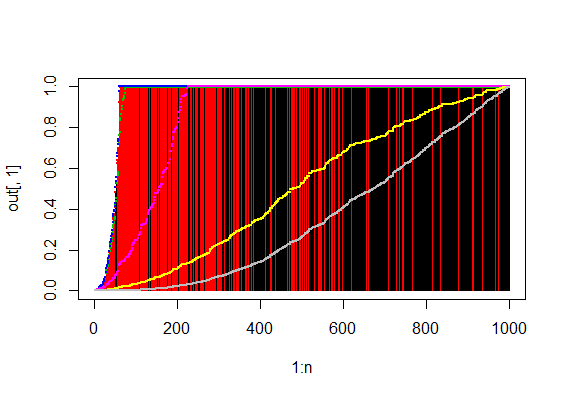
# Black:  null hypothesis.
# Red:  alternative hypothesis.
# 黒は帰無仮説が真、赤は対立仮説が真の場合のq値
# Increasing lines are q values from 6 methods
# 増加折れ線は６補正法のq値
plot(1:n,out[,1],pch=20,cex=0.1,col=col.ord,type="h")
for(i in 1:length(out[1,])){
	points(1:n,out[,i],pch=20,cex=0.5,col=i)
}
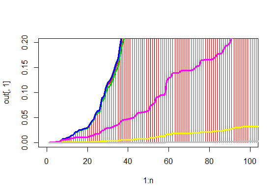
# Magnified plot with low q values.
# 低q valueの拡大図
plot(1:n,out[,1],pch=20,col=col.ord,type="h",xlim = c(0,100),ylim=c(0,0.2))
for(i in 1:length(out[1,])){
	points(1:n,out[,i],pch=20,lwd=3,col=i,type="l")
}