第四章: エントロピー、相対エントロピー、相互情報
最終更新:ID:bfG2vUKdOA 2015年07月16日(木) 17:54:47履歴
Summary 
この章では以下の話題に関する説明をしていきます.
これらの話が以後に続く説明の基本になる部分なので,一通りさらえるようにしておきます.
まず,情報というもの (これが,この講義のメイントピックです) の尺度に関する話をします.
結論から言ってしまえばエントロピーこそが,情報を扱う際の一つの基準になるということを話ます.
このエントロピーは後述する通り,基本的に確立の応用に過ぎません.
確率が,同時確率や,条件付き確率という応用をするようにエントロピーに関しても
結合エントロピーや条件付きエントロピーという概念を導入します.
これは基本的に確立のものをエントロピーの式に当てはめたものに過ぎません.
エントロピー関連の話題の最後に KLD: Kullback Leiber Distance の話をします.
上にも記述した通り, エントロピーは情報を扱う上での一つの基準です.
基準であるということは,2つのエントロピー同士を比較することができる(つまり距離である)必要があります.
KLD というのは,ここでいうエントロピー間の距離に相当します.
続いて, 相互情報量という話題に触れます.
これは, 2つの確率変数の相互依存の尺度を表す量のことです.
より直感的な説明をするなら, ある事象が判明した場合に, どの程度別のある事象が共起しておきるのかを示した値ということになるかと思います.
これを整理していくと Chain Rules というものが出てくることになります.
上記2つはエントロピーの表し方に関する説明になるわけですが,
その後, 離散確率分布のエントロピー に対する以下に示す 3 + 1 個の式を紹介します.
ここで紹介する式はいずれも不等式を利用します.
情報理論に於いては等式を使用することよりも不等式を使用することのほうが多いので式の導出,証明になれるとよいでしょう.
上記式のうち,講義の中で最も重要なのは Fano’s Inequality です.
これらの話が以後に続く説明の基本になる部分なので,一通りさらえるようにしておきます.
まず,情報というもの (これが,この講義のメイントピックです) の尺度に関する話をします.
結論から言ってしまえばエントロピーこそが,情報を扱う際の一つの基準になるということを話ます.
このエントロピーは後述する通り,基本的に確立の応用に過ぎません.
確率が,同時確率や,条件付き確率という応用をするようにエントロピーに関しても
結合エントロピーや条件付きエントロピーという概念を導入します.
これは基本的に確立のものをエントロピーの式に当てはめたものに過ぎません.
エントロピー関連の話題の最後に KLD: Kullback Leiber Distance の話をします.
上にも記述した通り, エントロピーは情報を扱う上での一つの基準です.
基準であるということは,2つのエントロピー同士を比較することができる(つまり距離である)必要があります.
KLD というのは,ここでいうエントロピー間の距離に相当します.
続いて, 相互情報量という話題に触れます.
これは, 2つの確率変数の相互依存の尺度を表す量のことです.
より直感的な説明をするなら, ある事象が判明した場合に, どの程度別のある事象が共起しておきるのかを示した値ということになるかと思います.
これを整理していくと Chain Rules というものが出てくることになります.
上記2つはエントロピーの表し方に関する説明になるわけですが,
その後, 離散確率分布のエントロピー に対する以下に示す 3 + 1 個の式を紹介します.
ここで紹介する式はいずれも不等式を利用します.
情報理論に於いては等式を使用することよりも不等式を使用することのほうが多いので式の導出,証明になれるとよいでしょう.
- Information Inequalities
- Log Sum Inequality
- Data Processing Inequality
- Fano’s Inequality
上記式のうち,講義の中で最も重要なのは Fano’s Inequality です.
Information Measures
まず,情報理論が相手にする情報というものに関して,これを量的に測る基準を
考えていきます.この基準としてデファクトスタンダードに使用されているものがエントロピーです.
Entropy
定義 4.1.1: Entropy
離散確立変数 X のエントロピー H(X) は以下の式によって求められます.
%20%3D%20-%20%5Csum_%7Bx%20%5Cin%20X%7D%20p(x)%20%5Clog(x)%0A%5C%5C%0Awhere%20%5C%20with%20%5C%20the%20%5C%20limit:%200%20%5Clog%200%20%3D%200.png)
細かいことはいいんだよ的に何をやっているのかのみを把握するなら,
p(x) をすべての事象分,足し合わせたものという認識をしてしまえばいいかと思います.
- p(x) log p(x) という形にしているのは場合の数を足し算で計算するため
- このままでは負になるので最後にマイナスをかけています
- そのため, エントロピーは定義上,負の値にはなりえません.
対数の底に関しては,所詮定数になるだけなので,本質的ではありませんが,
情報論の中では一般に 2 を使用します(単純にコンピュータは 0 1 ですので).
この場合 H(X) の単位は bit と呼ばれます.
しかし,別に 2 に限定する必要があるわけではなく, 例えば e をとる場合もあります.
この場合は nats をいう単位で記述します.
定義 4.1.2: Entropy
上記の定義は以下のように記述する場合もあります.
%20%3D%20-%20E_p%20%5Cbegin%7Bbmatrix%7D%0A%5Clog%20p(x)%0A%5Cend%7Bbmatrix%7D%20%3D%20E_p%20%5Cbegin%7Bbmatrix%7D%0A%5Clog%20%5Cfrac%7B1%7D%7Bp(x)%7D%0A%5Cend%7Bbmatrix%7D%20.png)
ようは, それぞれの個別具体的な確率 p(x) を足すのではなく,
その確率分布の期待値でまとめてしまっているだけですね.
- ここで E は 分布 p の期待値です.
Property 4.1.1: Logarithm
対数の性質には以下のようなものがあります.
%20%3D%20%5Clog_%7Bb%7D%20%5C%20a%20%5Clog_%7Ba%7D%20p(x).png)
これをエントロピーの定義に当てはめると以下のようになります.
%20%3D%20(log_%7Bb%7D%20%5C%20a)%20H_%7Ba%7D%20(X).png)
そのため,
%20%3D%20-p(X)log_y%20p(X).png) は y = a か b を保持することになります.
は y = a か b を保持することになります. Example 4.1.1: Binary Random Variable
ちょっと簡単な例を上げておきます.
%20%5C%5C%0A0%20%26%20(%5C%20with%20%5C%20probability%5C%20%20p)%20%5C%5C%0A%5Cend%7Barray%7D%20%5Cright..png)
この際のエントロピーは x=1 の場合と, x=0 の場合を足せばいいので,以下のようになります.
%20%3D%20(-p%20%5Clog%20p)%20+%20(%20-(1%20-%20p)%20%5Clog(1%20-%20p)).png)
しばしば, 上記の定義にしたがってエントロピーは以下のようになる場合があります.
%20%3D%20H(p).png)
Example 4.1.1 の確率変数のエントロピー H(p) は p の関数として記述することができます.
図を挿入
この際のエントロピーは x=1 の場合と, x=0 の場合を足せばいいので,以下のようになります.
しばしば, 上記の定義にしたがってエントロピーは以下のようになる場合があります.
Example 4.1.1 の確率変数のエントロピー H(p) は p の関数として記述することができます.
図を挿入
- 観察:
- (1) エントロピーは p が 0 or 1 の時はエントロピーは 0 になります.これは p=0, or p=1 の時には確率変数にランダム性はなく,不明瞭性もないからです.
- (2) エントロピーの最大値は p = 1/2 の時であり,これは,この時の不明瞭性が最大だからです.
Example 4.1.2:
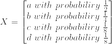
%20%26%3D%26%20-%20%5Cfrac%7B1%7D%7B2%7D%20%5Clog%20%5Cfrac%7B1%7D%7B2%7D%0A%20%20%20%20%20%20%20%20%20-%20%5Cfrac%7B1%7D%7B4%7D%20%5Clog%20%5Cfrac%7B1%7D%7B4%7D%0A%20%20%20%20%20%20%20%20%20-%20%5Cfrac%7B1%7D%7B8%7D%20%5Clog%20%5Cfrac%7B1%7D%7B8%7D%0A%20%20%20%20%20%20%20%20%20-%20%5Cfrac%7B1%7D%7B8%7D%20%5Clog%20%5Cfrac%7B1%7D%7B8%7D%20%5C%5C%0A%20%20%20%20%20%26%3D%26%20%5Cfrac%7B7%7D%7B4%7D.png)
例題 1:
一様分布をもつ32通り以上の確率変数を考えよ.
結果を特定するために,我々は32の異なった値を取るラベルが必要である.
- 要は,32 種類の記号を 0,1 で表す際に,位はいくつ必要かという問題っぽい.
(1) 結果をユニークに特定するためにどの程度のラベルが必要であるか?

そのため,5つのラベルが必要
- (2) 確率変数のエントロピーを計算せよ
%20%26%3D%26%20-%20%5Csum%5E%7B32%7D_%7Bi%3D1%7D%20p(i)%20%5Clog%7Bp(i)%7D%20%5C%5C%0A%20%20%20%20%20%26%3D%26%20-%20%5Csum%5E%7B32%7D_%7Bi%3D1%7D%20%5Cfrac%7B1%7D%7B32%7D%20%5Clog%7B%5Cfrac%7B1%7D%7B32%7D%7D%20%5C%5C%0A%20%20%20%20%20%26%3D%26%20%5Clog%7B32%7D%20%5C%5C%0A%20%20%20%20%20%26%3D%26%205%20%5C%20bit.png)
- (3) 結果は互いに一致するかを答えよ
上記の通り,一致する.
ただし,これはすべてのラベルが同じ長さを持つ場合の話です.
続いては,一様分布ではない例を考えます.
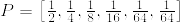
例題2: Horse Race
8頭の馬が参加している競馬があるとします.
ここで,それぞれの馬の勝率は以下のように定義されます.
- (1) 結果を一意に決めるためにはいくつのラベルが必要か?
3bit
- (2) Calculate the entropy of the random variable.
%20%26%3D%26%20%0A-%20%5Cfrac%7B1%7D%7B2%7D%20%5Clog%7B%5Cfrac%7B1%7D%7B2%7D%7D%0A-%20%5Cfrac%7B1%7D%7B4%7D%20%5Clog%7B%5Cfrac%7B1%7D%7B4%7D%7D%0A-%20%5Cfrac%7B1%7D%7B8%7D%20%5Clog%7B%5Cfrac%7B1%7D%7B8%7D%7D%0A-%20%5Cfrac%7B1%7D%7B16%7D%20%5Clog%7B%5Cfrac%7B1%7D%7B16%7D%7D%0A-%204%20%5Cfrac%7B1%7D%7B64%7D%20%5Clog%7B%5Cfrac%7B1%7D%7B64%7D%7D%5C%5C%0A%26%3D%26%202%20%5C%20bit.png)
- (3) 上記の結果は一致しているか? 一致していない場合,どのようにすれば,ラベルの平均長を最小にできるのか?
一致はしない.そのため,勝率が最も高い馬から短いラベルを振っていく.
- (4) あなたはレースの結果をしらないので,知っている誰かに結果を聞くとします.
- レースで勝利した馬がどれかを知るためには平均で何回の質問する必要がありますか?
- ただし,ここで行える必要は yes-no クエスチョンであるとします.
Joint Entropy and Conditional Entropy
定義 4.1.3: Joint Entropy
The joint entropy H(X, Y) of discrete random variables X and Y is defined by:
H X , Y p x , y log p x , y E p log p x , y
x X y Y
where E p is the expectation with respect to the joint distribution p.
Note that H(X,Y) does NOT take negative values.
定義 4.1.4: Conditional Entropy
If discrete random variables X and Y follow the joint distribution p(x, y),
conditional entropy H(Y|X) is defined as:
H Y X p x H Y X x p x p y x log p y x
x X
x X
y Y
p x p y x log p y x p x , y log p y x E p ( x , y ) log p Y X
Theorem 4.1.1: Chain Rule
H X , Y H X H Y X
Proof:
H ( X , Y ) p x , y log p x , y p x , y log p ( x ) p y x
x X y Y
x X y Y
p x , y log p x
x X y Y
p ( x ) log p ( x )
x X
p x , y log p y x
x X y Y
p x , y log p y x
x X y Y
H ( X ) H ( Y X )
Corollary 4.1.1: Chain Rule in Probability Domain
log p X , Y log p X log p Y X
Proof: Obvious from the conditional probability rule.
Corollary 4.1.2: H X , Y Z H X Z H Y X , Z
Proof: Obvious from the chain rule.
Remark: H X Y H Y X
However, H X H X Y H Y H Y X
( I ( X , Y ) : Mutual
Informatio n )
Example 4.1.3:
Let random variables x , y 1 ,
2 , 3 , 4
have the following joint distribution:
x
1 1
8 16
1 1
p ( X x , Y y ) 16 8
1 1
16 16
1
0
4
1
32
1
32
1
16
0
1
32
1
32
1
16
0
y
Example 4.1.3 (Continued):
Then, the marginal probability of X and Y are:
1
p ( X x )
2
1
4
1
8
1
8
and
1
p ( Y y )
4
1
4
1
4
1
4
Hence, H(X)=7/4 bits and H(Y)=2 bits. The conditional entropy H(X|Y) is:
4
11
H X Y p ( Y y ) H ( X Y y )
bits,
8
y 1
and the conditional entropy H(Y|X) is:
4
13
H Y X p ( X x ) H ( Y X x )
8
x 1
bits.
The joint entropy H(X,Y) is:
4
4
H X , Y p ( X x , Y y ) log p ( X x , Y y )
x 1 y 1
27
8
bits.
Kullback Leiber Distance (Relative Entropy)
定義 4.1.5: Kullback Leiber Distance
The Kullback Leiber distance D(p || q) between the two probability distribution
functions p(x) and q(x) is defined as:
D p q p ( x ) log
0
q
with 0 log 0
x X
,
p log
p
.
0
p ( x )
p ( X )
E p log
q ( x )
q ( X )
Property 4.1.2: Distance between Probability Distrib
(1)
(2)
(3)
(4)
D ( p q ) D ( q p )
in general
D(p || q) is non-negative, and is zero if and only if p=q for all x.
The Kullback Leiber distance is sometimes called relative entropy.
If the probability distribution q, which is believed to be correct,
is different from the true distribution p, we need
H ( p ) D ( p q )
bits on the average to describe the random variable following p.
Mutual Information
定義 4.2.1: Mutual Information
Consider two random variables X and Y with a joint probability distribution
function p(x,y) and the marginal distributions p(x) and p(y). The mutual
Information I(X,Y) is the relative entropy between the joint distribution and
the product distribution p(x)p(y), i.e.,
I X ; Y p ( x , y ) log
x X y Y
p ( x , y )
p ( x ) p ( y )
p ( X , Y )
D p ( x , y ) p ( x ) p ( y ) E p ( x , y ) log
p
(
X
)
p
(
Y
)
Theorem 4.2.1: Entropy and Mutual Information
I X ; Y H ( X ) H ( X Y )
Observation:
The mutual information I(X,Y) is the reduction in the uncertainty of X by
knowing Y.
Exercise: Give a proof for Theorem 4.1.2
Corollary 4.2.1:
Proof: Obvious from the 定義.
Corollary 4.2.2: I X ; Y H X H Y H X , Y
Proof: Obvious from the 定義.
I X ; X H X H X X H ( X )
Corollary 4.2.3:
Proof: Obvious from the 定義.
Theorem 4.2.2: Extension of the Chain Rule
Let X 1 , X 2 ,..., X n be random variables drawn from the joint distribution
p(x 1 , x 2 ,..., x n ). Then,
n
H X 1 , X 2 , , X n H X i X i 1 , , X 1
Proof:
i 1
H X 1 , X 2 H X 1 H X 2 X 1
H X 1 , X 2 , X 3 H X 1 H X 2 , X 3 X 1
H X 1 H X 2 X 1 H X 3 X 2 , X 1
By continuing the process, we have:
H X 1 , X 2 , , X n H X 1 H X 2 X 1 H X n X n 1 , , X 1
n
H X i X i 1 , , X 1
定義 4.2.2: Conditional Mutual Information
Conditional mutual information of random variable X and Y , given Z is
defined by:
I X ; Y Z H ( X Z ) H ( X Y , Z )
p ( X , Y Z )
E p ( x , y , z ) log
p
(
X
Z
)
p
(
Y
Z
)
Theorem 4.2.3: Chain Rule for Mutual Information
n
I X 1 , X 2 , , X n ; Y I X i ; Y X i 1 , X i 2 , , X 1
Proof:
i 1
I X 1 , X 2 , , X n ; Y H X 1 , X 2 , , X n H X 1 , X 2 , , X n Y
n
H X i X i 1 , , X 1
i 1
n
n
H X
i 1
I X i ; Y X 1 , X 2 , , X i 1
Theorem 4.2.4: Non-Negativity of Mutual Informat
I X ; Y 0
with equality if and only if X and Y are independent.
Proof: I X ; Y D p ( x , y ) p ( x ) p ( y ) 0
with equality if and only if p(x,y)= p(x) p(y) , i.e., X and Y are independent.
Theorem 4.2.5: Non-Negativity of Conditional
Mutual Information
I X ; Y Z 0
with equality if and only if X and Y are conditionally independent given Z.
Proof: Obvious from the 定義 of the conditional mutual information.
Theorem 4.2.6: Entropy with Uniform
Distribution
Let X
denote the number of the elements in a set X. Then,
H X log X
with equality if and only of x has a uniform distribution over X.
Proof: Let u(x)=1/|X| be the uniform probability distribution function over X,
and let p(x) be the probability distribution for X. Then,
p ( x )
D p u p ( x ) log
log X H ( X )
u ( x )
Hence, by the non-negativity of relative entropy,
0 D p u log X
H ( X )
Theorem 4.2.7: Conditioning reduces entropy
H X Y H ( X )
holds, with equality if and only if X and Y are independent.
Proof:
0 I X ; Y H ( X ) H ( X Y )
Theorem 4.2.8: Independence Bound on entropy
Let X 1 , X 2 ,..., X n be random variables drawn from the joint distribution
n
p(x 1 , x 2 ,..., x n ). Then,
H X 1 , X 2 , , X n H X i
i 1
Proof:
n n
i 1 i 1
H X 1 , X 2 , , X n H X i X i 1 , , X 1 H X i
Chain Rules
Information Inequalities
Theorem 4.3.1: Log Sum Inequality
For non-negative numbers, a 1 , a 2 , ...., a n and
b 1 , b 2 , ...., b n ,
n
a i
n
a i n
a i log a i log i n 1
b i i 1
i 1
b i
a i
constant
with equality if and only if
b i
i 1
for any
i
Proof: The function f(t)=t log t is strictly convex, since f’’(t)=(1/t)loge>0
for all positive t. Therefore, by Jensen’s inequality, we have
f t f t
and
Setting b / b
i
i
i i
for i 0 ,
i
j
t i a i / b i
j 1
We have:
a i
log
n
b
j 1
j
i
i
n
i
,
a i
a
a
n i log n i
b i
b j
b j
Theorem 4.3.2: Convexity of Relative Entropy
D(p || q) is convex in the pair (p,q), i.e., if (p 1 ,q 1 ), (p 2 ,q 2 ), are two pairs of the
probability distribution of x X ,
D p 1 ( 1 ) p 2 q 1 ( 1 ) q 2 D p 1 q 1 ( 1 ) D p 2 q 2 , 0 1
Proof:
Applying the log sum inequality to the terms on LHS and RHS,
p 1 ( x ) ( 1 ) p 2 ( x )
p 1 ( 1 ) p 2 log
q 1 ( x ) ( 1 ) q 2 ( x )
p ( x )
( 1 ) p 2 ( x )
p 1 ( x ) log 1 ( 1 ) p 2 ( x ) log
q 1 ( x )
( 1 ) q 2 ( x )
Summing this over all x X , we obtain the equation shown in the theorem.
定義 4.3.1: Concavity
A function f is concave, if –f is convex.
Theorem 4.3.3: Concavity of Entropy
H(p) is a concave function of p.
Proof:
H p log X
D p u
where u is the uniform distribution having cardinality |X|.
Then the concavity of H(p) is obvious.
Theorem 4.3.4: Concavity of Mutual Information
Let X and Y be random variables having a joint distribution p(x,y)= p(x) p(y|x).
Mutual information I(X;Y) is a concave function of p(x) for fixed p(y|x), and
a convex function of p(y|x) for fixed p(x).
Proof:
I ( X , Y ) H ( Y ) H ( Y | X ) H ( Y )
p ( x ) H ( Y | X x )
Theorem 4.3.4 (Proof continued-1):
If p(y|x) is fixed, then H ( Y | X ) is fixed.
Also, because p(y|x) is fixed, p(y) is a linear function of p(x).
Since H(Y) is a concave function of p(y), it is also a concave function of p(x).
Now, let’s consider two different conditional probability distribution p 1 (y|x)
and p 2 (y|x), with which the corresponding joint probabilities are:
p 1 (y,x)=p(x) p 1 (y|x) and p 2 (y,x)=p(x) p 2 (y|x), and their marginals being
p(x) and p 1 (y), and p(x) and p 2 (y), respectively.
Consider conditional, conditional, and marginal distributions:
p ( y x ) p 1 ( y x ) ( 1 ) p 2 ( y x )
p ( y , x ) p 1 ( y , x ) ( 1 ) p 2 ( y , x )
p ( y ) p 1 ( y ) ( 1 ) p 2 ( y )
Theorem 4.3.4 (Proof continued-2):
Define q ( x , y ) p ( x ) p ( y )
Obviously, q ( x , y ) q 1 ( x , y ) ( 1 ) q 2 ( x , y )
Since the mutual information is Kullback Leibler distance between the joint
distribution and the product of the marginals,
I ( X ; Y ) D p q
and since the Kullback Leibler distance (=relative entropy) is a convex
function of (p, q), it follows that the mutual information is a convex function
of the conditional distribution.
Log Sum Inequality
Data Processing Inequality
定義 4.4.1: XYZ
Random variables X, Y, Z are said to form a Markov Chain in the order
XYZ, if the joint probability follows:
p ( x , y , z ) p ( x ) p ( y x ) p ( z y )
Property 4.4.1:
(1) XYZ if and only if X and Z are conditionally independent of Y given,
i.e.,
p ( x , y , z ) p ( x , y ) p ( z y )
p ( x , z y )
p ( x y ) p ( z y )
p ( y )
p ( y )
(2) XYZ implies ZYX.
(3) If Z=f(Y), then XYZ .
Theorem 4.4.1: Data Processing Inequality
If XYZ, then I ( X ; Y ) I ( X ; Z )
Proof:
Since I ( X ; Y , Z ) I ( X ; Z ) I ( X ; Y Z ) I ( X ; Y ) I ( X ; Z Y )
However, since X and Z are conditionally independent of Y given,
I ( X ; Z Y ) 0
Since I ( X ; Y Z ) 0 , we have: I ( X ; Y ) I ( X ; Z ) .
Corollary 4.4.1:
I ( Y ; Z ) I ( X ; Z )
Proof: Obvious from the 定義.
Corollary 4.4.2:
If XYZ=f(Y), then I ( X ; Y ) I ( X ; f ( Y )) Proof: Obvious from the 定義.
Function does not increase information!!!
Corollary 4.4.3:
If XYZ, then I ( X ; Y Z ) I ( X ; Y ) Proof: Obvious from the 定義.
Observation reduces the dependence of the random variables!!!
Fano’s Inequality
Consider a very simple communication system described below:
Source
X
+
Y
Estimator
g(Y)
X ˆ g ( Y )
Noise = Error source
From the received signal Y, the estimator g(Y) estimates the transmitted
source X.
Faon’s inequality specifies the bound of the probability of error: P e =Pr( X ˆ X )
Theorem 4.5.1: Fano’s Inequality
H ( P e ) P e log X
1 H ( X Y )
Proof: Define variable corresponding to the error event:
1
E
0
if
if
X ˆ X
X ˆ X
Using the chain rule for entropies, we can expand H(E,X|Y) in the
following two ways:
Theorem 4.5.1 (Proof continued-1):
H ( E , X Y ) H ( X Y ) H ( E X , Y ) H ( E Y ) H ( X E , Y )
0
H ( P e )
(a)
(b)
P e log X
(c)
1
(a) Since E is a function of X and g(Y), if the receiver knows X, Y and g(Y) as
conditions of E, there is no uncertainty on E, and hence this term is zero.
(b) Since conditioning reduces entropy, H ( E Y ) H ( E ) H ( P e )
(c) This term is bounded as:
H ( X E , Y ) Prob ( E 0 ) H ( X Y , E 0 ) Prob ( E 1 ) H ( X Y , E 1 )
0
(d)
log X
1
(e)
(d) Since given E=0, X=g(Y) is known. Therefore, there is no uncertainty.
(e) Given E=1, we can upper-bound the conditional entropy by the
logarithm of the remaining outcomes |X|-1.
Combining these results, we obtain Fano’s inequality.
Corollary 4.5.1: Wider Sense of Fano’s Inequality
1 P e log X
H ( X Y )
or
P e
H ( X Y ) 1
log X
Proof: In the proof of Theorem 4.1.16, (b) and (e) can further be
upper-bounded by
H ( X Y ) H ( E Y ) H ( X E , Y )
H ( P e ) 1
(b’)
1
(c)
H ( X E , Y ) P e log X
(e)
respectively.
P e log X
1 P e log X
(e’)
Quiz
Illustrative Example: Weather in Kanazawa and Fukui
Shine Rain
Fukui
Kanazawa
P(x,y) Rain Shine
0.445 0.055
0.055 0.445
Shine Rain
Fukui
Kanazawa
P(x,y) Rain Shine
0.445 0.055
0.055 0.445

コメントをかく